Quickstart

Installation

Refer to the Installation page for instructions on how to install comyx.

Getting Started

The following example demonstrates the use of Comyx to simulate a simple wireless network. Note that the following example is the same as the first example in the examples page.

System Model

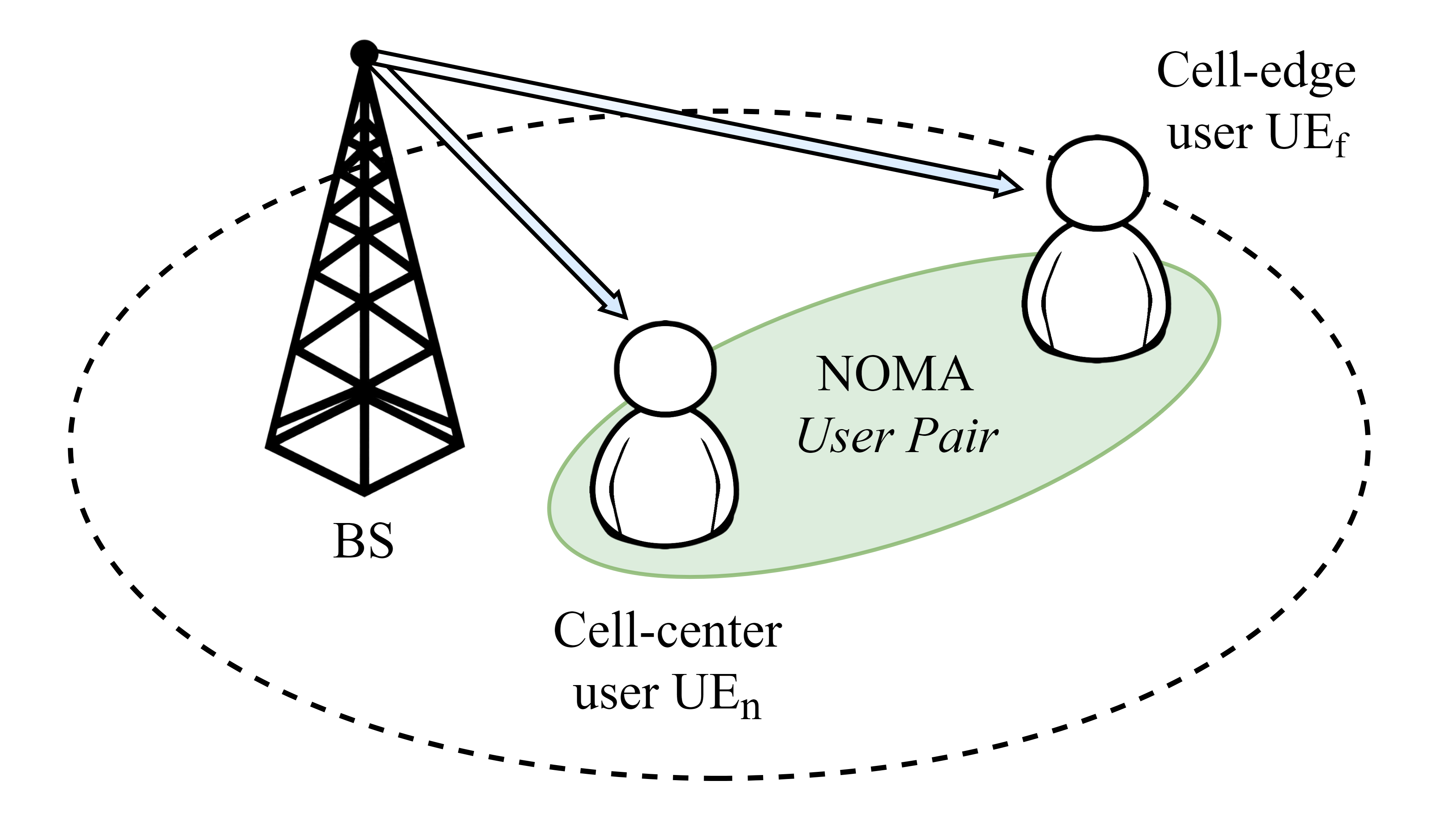
Consider a simple downlink NOMA system with a single base station (\(\mathrm{BS}\)), a cell-center user (\(\mathrm{UE}_n\)) and a cell-edge user (\(\mathrm{UE}_f\)).

For the sake of simplicity, assume that both base station and users are equipped with a single antenna.

Fig. 1. Downlink NOMA system model.

Let \(x_n\) and \(x_f\) denote the messages intended for \(\mathrm{UE}_n\) and \(\mathrm{UE}_f\), respectively. The \(\mathrm{BS}\) transmits a superposition of the two messages weighted by the power allocation coefficients \(\alpha_n\) and \(\alpha_f\), respectively. Mathematically, the transmitted signal can be expressed as

\[ x = \sqrt{\alpha_n P_t} x_n + \sqrt{\alpha_f P_t} x_f, \]

where \(P_t\) is the transmit power of the \(\mathrm{BS}\).

In NOMA, successive interference cancellation (SIC) is employed at the users to decode their intended messages. The optimal decoding order is in the order of increasing channel gains. Let \(h_n\) and \(h_f\) denote the channel gains of \(\mathrm{UE}_n\) and \(\mathrm{UE}_f\), respectively, then, for the present case, \(|h_n|^2 > |h_f|^2\). As such, \(\mathrm{UE}_n\) decodes the message intended for \(\mathrm{UE}_f\) first and then cancels it from the received signal to decode its own message, while \(\mathrm{UE}_f\) decodes its own message directly. Furthermore, the received signal at \(\mathrm{UE}_i\), \(i \in \{n, f\}\), can be expressed as

\[ y_i = h_i x + n_i, \]

where \(n_i\) is the additive white Gaussian noise (AWGN) at \(\mathrm{UE}_i\) with zero mean and variance \(\sigma_i^2\).

Assuming perfect SIC, the achievable rates at \(\mathrm{UE}_n\) and \(\mathrm{UE}_f\) are given by

\[\begin{split} \begin{align*} R_{n\,\rightarrow\,f} &= \log_2 \left(1 + \frac{\alpha_f P_t |h_n|^2}{\alpha_n P_t |h_n|^2 + N_0}\right),\\ R_n &= \log_2 \left(1 + \frac{\alpha_n P_t |h_n|^2}{N_0}\right), \\ \end{align*} \end{split}\]

and

\[ R_f = \log_2 \left(1 + \frac{\alpha_f P_t |h_f|^2}{\alpha_n P_t |h_f|^2 + N_0}\right), \]

where \(N_0\) is the noise power spectral density, and \(R_{f\,\rightarrow\,n}\) is the achievable data rate at \(\mathrm{UE}_n\) before SIC.

Simulation

In this example, we will simulate the downlink NOMA system described above. First, we import the necessary modules.

from comyx.network import UserEquipment, BaseStation
from comyx.core import SISOCollection
from comyx.propagation import get_noise_power
from comyx.utils import dbm2pow, get_distance

import numpy as np
from numba import jit
from matplotlib import pyplot as plt

plt.rcParams["font.family"] = "STIXGeneral"
plt.rcParams["figure.figsize"] = (6, 4)

Here, we import numba to drastically increase the simulation loop speed. Next, we define the simulation parameters.

Pt = np.linspace(-10, 30, 80)  # dBm
Pt_lin = dbm2pow(Pt)  # Watt
bandwidth = 1e6  # Bandwidth in Hz
frequency = 2.4e9  # Carrier frequency
temperature = 300  # Kelvin
mc = 100000  # Number of channel realizations

N0 = get_noise_power(temperature, bandwidth)  # dBm
N0_lin = dbm2pow(N0)  # Watt

fading_args = {"type": "rayleigh", "sigma": 1 / 2}
pathloss_args = {
    "type": "reference",
    "alpha": 3.5,
    "p0": 20,
    "frequency": frequency,
}  # p0 is the reference power in dBm

Refer to API reference for more information on the pathloss and fading models.

Next, we define the users and the base station.

BS = BaseStation("BS", position=[0, 0, 10], n_antennas=1, t_power=Pt_lin)
UEn = UserEquipment("UEn", position=[200, 200, 1], n_antennas=1)
UEf = UserEquipment("UEf", position=[400, 400, 1], n_antennas=1)

print("Distance between BS and UEn:", get_distance(BS.position, UEn.position))
print("Distance between BS and UEf:", get_distance(BS.position, UEf.position))

Distance between BS and UEn: 282.98586537139977
Distance between BS and UEf: 565.7570149808131

Here, t_power is the transmit power of the base station. It could have been either in dBm or Watt. comyx aims to be low-level and modular, and therefore, it expects the user to keep track of the units. In this example, we have used Watt as the unit for power.

Now, we define a core component of comyx called SISOCollection. This component is responsible for generating the channel realizations as per the provided pathloss and fading arguments.

link_col = SISOCollection(realizations=mc)

# Add links to the collection
link_col.add_link([BS, UEn], fading_args, pathloss_args)
link_col.add_link([BS, UEf], fading_args, pathloss_args)

As mentioned in the system model section, the achievable rates at \(\mathrm{UE}_n\) and \(\mathrm{UE}_f\) are given by

\[ R_n = \log_2 \left(1 + \frac{\alpha_n P_t |h_n|^2}{N_0}\right), \]

and

\[ R_f = \log_2 \left(1 + \frac{\alpha_f P_t |h_f|^2}{\alpha_n P_t |h_f|^2 + N_0}\right). \]

As this notebook intends to give a simple illustration of NOMA, we assume that the power allocation coefficients are fixed.

In particular, we set \(\alpha_n = 0.25\) and \(\alpha_f = 0.75\).

BS.allocations = {"UEn": 0.25, "UEf": 0.75}

Now, we can write the simulation loop and compute the achievable rates as per the above equations.

UEn.sinr_pre = np.zeros((len(Pt), mc))
UEn.sinr = np.zeros((len(Pt), mc))
UEf.sinr = np.zeros((len(Pt), mc))

# Get channel gains
gain_f = link_col.get_magnitude("BS->UEf") ** 2
gain_n = link_col.get_magnitude("BS->UEn") ** 2

for i, p in enumerate(Pt_lin):
    p = BS.t_power[i]

    # Edge user
    UEf.sinr[i, :] = (BS.allocations["UEf"] * p * gain_f) / (
        BS.allocations["UEn"] * p * gain_f + N0_lin
    )

    # Center user
    UEn.sinr_pre[i, :] = (BS.allocations["UEf"] * p * gain_n) / (
        BS.allocations["UEn"] * p * gain_n + N0_lin
    )
    UEn.sinr[i, :] = (BS.allocations["UEn"] * p * gain_n) / N0_lin


rate_nf = np.log2(1 + UEn.sinr_pre)
rate_n = np.log2(1 + UEn.sinr)
rate_f = np.log2(1 + UEf.sinr)

# Rate thresholds
thresh_n = 1
thresh_f = 1

# JIT compiled as mc can be very large (>> 10000)
@jit(nopython=True)
def get_outage(rate_nf, rate_n, rate_f, thresh_n, thresh_f):
    outage_n = np.zeros((len(Pt), 1))
    outage_f = np.zeros((len(Pt), 1))

    for i in range(len(Pt)):
        for k in range(mc):
            if rate_nf[i, k] < thresh_f or rate_n[i, k] < thresh_n:
                outage_n[i] += 1
            if rate_f[i, k] < thresh_f:
                outage_f[i] += 1

    return outage_n, outage_f

UEn.outage, UEf.outage = get_outage(rate_nf, rate_n, rate_f, thresh_n, thresh_f)
UEn.outage /= mc
UEf.outage /= mc

UserEquipment has a property called rate which computes the achievable rate as per the following equation of Shannon’s capacity theorem. Note that the property also takes the mean of the achievable rates over the channel realizations along the last axis (-1), if not specified otherwise.

\[ R = \log_2 \left(1 + \mathrm{SINR}\right). \]

Finally, we can plot the results; the achievable rate and the outage probability.

plot_args = {
    "markevery": 10,
    "color": "k",
    "markerfacecolor": "r",
}

# Plot achievable rates
plt.figure()
plt.plot(Pt, UEn.rate, label="Rate UE$_n$", marker="s", **plot_args)
plt.plot(Pt, UEf.rate, label="Rate UE$_f$", marker="d", **plot_args)
plt.xlabel("Transmit power (dBm)")
plt.ylabel("Rate (bps/Hz)")
plt.grid(alpha=0.25)
plt.legend()
plt.show()

Fig. 2. Achievable rates at the users.

plot_args = {
    "markevery": 10,
    "color": "k",
    "markerfacecolor": "c",
}

# Plot outage probabilities
plt.figure()
plt.semilogy(Pt, UEn.outage, label="Rate UE$_n$", marker="s", **plot_args)
plt.semilogy(Pt, UEf.outage, label="Rate UE$_f$", marker="d", **plot_args)
plt.xlabel("Transmit power (dBm)")
plt.ylabel("Outage probability")
plt.grid(alpha=0.25)
plt.legend()
plt.savefig("figs/dl_noma_op.png", dpi=300, bbox_inches="tight")
plt.close()

Fig. 3. Outage probabilities of the users.

Great! We have successfully simulated a downlink NOMA system. The plots are in line with our expectations. As the transmit power increases, both users observe an increase in their achievable rates, however, after a certain point, the rate of \(\mathrm{UE}_f\) saturates. This is because \(\mathrm{UE}_f\) is in the cell-edge and the achievable rate is limited by the channel gain.