
SISO Downlink NOMA#
System Model#
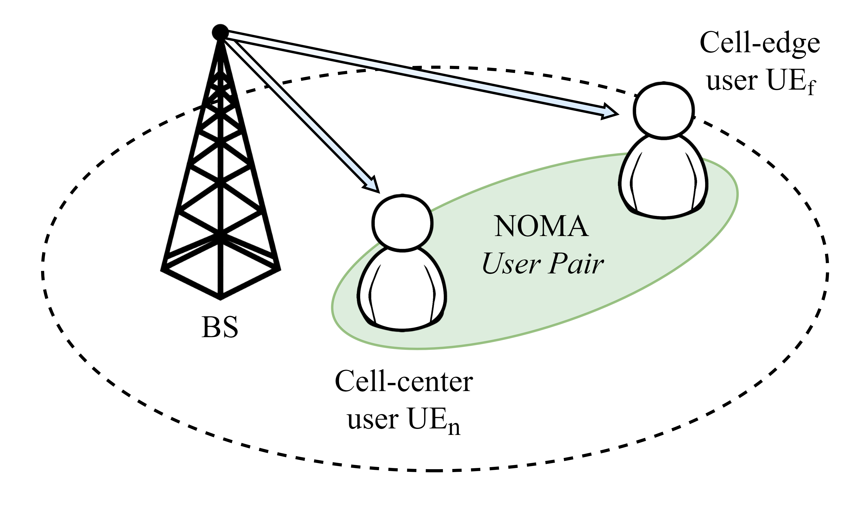
Consider a simple downlink NOMA system with a single base station (\(\mathrm{BS}\)), a cell-center user (\(\mathrm{UE}_n\)) and a cell-edge user (\(\mathrm{UE}_f\)).
For the sake of simplicity, assume that both base station and users are equipped with a single antenna.
Let \(x_n\) and \(x_f\) denote the messages intended for \(\mathrm{UE}_n\) and \(\mathrm{UE}_f\), respectively. The \(\mathrm{BS}\) transmits a superposition of the two messages weighted by the power allocation coefficients \(\alpha_n\) and \(\alpha_f\), respectively. Mathematically, the transmitted signal can be expressed as
where \(P_t\) is the transmit power of the \(\mathrm{BS}\).
In NOMA, successive interference cancellation (SIC) is employed at the users to decode their intended messages. The optimal decoding order is in the order of increasing channel gains. Let \(h_n\) and \(h_f\) denote the channel gains of \(\mathrm{UE}_n\) and \(\mathrm{UE}_f\), respectively, then, for the present case, \(|h_n|^2 > |h_f|^2\). As such, \(\mathrm{UE}_n\) decodes the message intended for \(\mathrm{UE}_f\) first and then cancels it from the received signal to decode its own message, while \(\mathrm{UE}_f\) decodes its own message directly. Furthermore, the received signal at \(\mathrm{UE}_i\), \(i \in \{n, f\}\), can be expressed as
where \(n_i\) is the additive white Gaussian noise (AWGN) at \(\mathrm{UE}_i\) with zero mean and variance \(\sigma_i^2\).
Assuming perfect SIC, the achievable rates at \(\mathrm{UE}_n\) and \(\mathrm{UE}_f\) are given by
and
where \(N_0\) is the noise power spectral density, and \(R_{f\,\rightarrow\,n}\) is the achievable data rate at \(\mathrm{UE}_n\) before SIC.
Simulation#
from comyx.network import UserEquipment, BaseStation, Link
from comyx.propagation import get_noise_power
from comyx.utils import dbm2pow, get_distance, generate_seed, db2pow


import numpy as np
from numba import jit
from matplotlib import pyplot as plt

plt.rcParams["font.family"] = "STIXGeneral"
plt.rcParams["figure.figsize"] = (6, 4)
Setup Environment#
Pt = np.linspace(-10, 30, 80)  # dBm
Pt_lin = dbm2pow(Pt)  # Watt
bandwidth = 1e6  # Bandwidth in Hz
frequency = 2.4e9  # Carrier frequency
temperature = 300  # Kelvin
mc = 100000  # Number of channel realizations

N0 = get_noise_power(temperature, bandwidth)  # dBm
N0_lin = dbm2pow(N0)  # Watt

n_antennas = 1

fading_args = {"type": "rayleigh", "sigma": 1 / 2}
pathloss_args = {
    "type": "reference",
    "alpha": 3.5,
    "p0": 20,
    "frequency": frequency,
}  # p0 is the reference power in dBm
BS = BaseStation("BS", position=[0, 0, 10], n_antennas=1, t_power=Pt_lin)
UEn = UserEquipment("UEn", position=[200, 200, 1], n_antennas=1)
UEf = UserEquipment("UEf", position=[400, 400, 1], n_antennas=1)

print("Distance between BS and UEn:", get_distance(BS.position, UEn.position))
print("Distance between BS and UEf:", get_distance(BS.position, UEf.position))
Distance between BS and UEn: 282.98586537139977
Distance between BS and UEf: 565.7570149808131
Initialize Links#
# Shapes for channels
shape_bu = (n_antennas, n_antennas, mc)

# Links
# fmt: off
link_bs_uen = Link(
    BS, UEn,
    fading_args, pathloss_args,
    shape=shape_bu, seed=generate_seed("BS-UEn"),
)

link_bs_uef = Link(
    BS, UEf,
    fading_args, pathloss_args,
    shape=shape_bu, seed=generate_seed("BS-UEf"),
)
Verify \(|h_n|^2 > |h_f|^2\)
np.mean(link_bs_uen.magnitude**2) > np.mean(link_bs_uef.magnitude**2)
np.True_
Compute Rates#
As mentioned earlier, the achievable rates at \(\mathrm{UE}_n\) and \(\mathrm{UE}_f\) are given by
and
As this notebook intends to give a simple illustration of NOMA, we assume that the power allocation coefficients are fixed.
In particular, we set \(\alpha_n = 0.25\) and \(\alpha_f = 0.75\).
BS.allocations = {"UEn": 0.25, "UEf": 0.75}

UEn.sinr_pre = np.zeros((len(Pt), mc))
UEn.sinr = np.zeros((len(Pt), mc))
UEf.sinr = np.zeros((len(Pt), mc))

# Get channel gains
gain_f = link_bs_uef.magnitude**2
gain_n = link_bs_uen.magnitude**2

for i, p in enumerate(Pt_lin):
    p = BS.t_power[i]

    # Edge user
    UEf.sinr[i, :] = (BS.allocations["UEf"] * p * gain_f) / (
        BS.allocations["UEn"] * p * gain_f + N0_lin
    )

    # Center user
    UEn.sinr_pre[i, :] = (BS.allocations["UEf"] * p * gain_n) / (
        BS.allocations["UEn"] * p * gain_n + N0_lin
    )
    UEn.sinr[i, :] = (BS.allocations["UEn"] * p * gain_n) / N0_lin


rate_nf = np.log2(1 + UEn.sinr_pre)
rate_n = np.log2(1 + UEn.sinr)
rate_f = np.log2(1 + UEf.sinr)

# Rate thresholds
thresh_n = 1
thresh_f = 1


# JIT compiled as mc can be very large (>> 10000)
@jit(nopython=True)
def get_outage(rate_nf, rate_n, rate_f, thresh_n, thresh_f):
    outage_n = np.zeros((len(Pt), 1))
    outage_f = np.zeros((len(Pt), 1))

    for i in range(len(Pt)):
        for k in range(mc):
            if rate_nf[i, k] < thresh_f or rate_n[i, k] < thresh_n:
                outage_n[i] += 1
            if rate_f[i, k] < thresh_f:
                outage_f[i] += 1

    return outage_n, outage_f


UEn.outage, UEf.outage = get_outage(rate_nf, rate_n, rate_f, thresh_n, thresh_f)
UEn.outage /= mc
UEf.outage /= mc
Results#
plot_args = {
    "markevery": 10,
    "color": "k",
    "markerfacecolor": "r",
}

# Plot achievable rates
plt.figure()
plt.plot(Pt, UEn.rate, label="Rate UE$_n$", marker="s", **plot_args)
plt.plot(Pt, UEf.rate, label="Rate UE$_f$", marker="d", **plot_args)
plt.xlabel("Transmit power (dBm)")
plt.ylabel("Rate (bps/Hz)")
plt.grid(alpha=0.25)
plt.legend()
plt.savefig("figs/dl_noma_rate.png", dpi=300, bbox_inches="tight")
plt.close()

plot_args = {
    "markevery": 10,
    "color": "k",
    "markerfacecolor": "c",
}

# Plot outage probabilities
plt.figure()
plt.semilogy(Pt, UEn.outage, label="Outage UE$_n$", marker="s", **plot_args)
plt.semilogy(Pt, UEf.outage, label="Outage UE$_f$", marker="d", **plot_args)
plt.xlabel("Transmit power (dBm)")
plt.ylabel("Outage probability")
plt.grid(alpha=0.25)
plt.legend()
plt.savefig("figs/dl_noma_op.png", dpi=300, bbox_inches="tight")
plt.close()
